
Seasonality, Holiday Effects, And Regressors
Modeling Holidays and Special Events
If you have holidays or other recurring events that you’d like to model, you must create a dataframe for them. It has two columns (holiday and ds) and a row for each occurrence of the holiday. It must include all occurrences of the holiday, both in the past (back as far as the historical data go) and in the future (out as far as the forecast is being made). If they won’t repeat in the future, Prophet will model them and then not include them in the forecast.
You can also include columns lower_window and upper_window which extend the holiday out to [lower_window, upper_window] days around the date. For instance, if you wanted to include Christmas Eve in addition to Christmas you’d include lower_window=-1,upper_window=0. If you wanted to use Black Friday in addition to Thanksgiving, you’d include lower_window=0,upper_window=1. You can also include a column prior_scale to set the prior scale separately for each holiday, as described below.
Here we create a dataframe that includes the dates of all of Peyton Manning’s playoff appearances:
1
2
3
4
5
6
7
8
9
10
11
12
13
14
15
16
17
18
19
# R
library(dplyr)
playoffs <- data_frame(
  holiday = 'playoff',
  ds = as.Date(c('2008-01-13', '2009-01-03', '2010-01-16',
                 '2010-01-24', '2010-02-07', '2011-01-08',
                 '2013-01-12', '2014-01-12', '2014-01-19',
                 '2014-02-02', '2015-01-11', '2016-01-17',
                 '2016-01-24', '2016-02-07')),
  lower_window = 0,
  upper_window = 1
)
superbowls <- data_frame(
  holiday = 'superbowl',
  ds = as.Date(c('2010-02-07', '2014-02-02', '2016-02-07')),
  lower_window = 0,
  upper_window = 1
)
holidays <- bind_rows(playoffs, superbowls)
1
2
3
4
5
6
7
8
9
10
11
12
13
14
15
16
17
18
# Python
playoffs = pd.DataFrame({
  'holiday': 'playoff',
  'ds': pd.to_datetime(['2008-01-13', '2009-01-03', '2010-01-16',
                        '2010-01-24', '2010-02-07', '2011-01-08',
                        '2013-01-12', '2014-01-12', '2014-01-19',
                        '2014-02-02', '2015-01-11', '2016-01-17',
                        '2016-01-24', '2016-02-07']),
  'lower_window': 0,
  'upper_window': 1,
})
superbowls = pd.DataFrame({
  'holiday': 'superbowl',
  'ds': pd.to_datetime(['2010-02-07', '2014-02-02', '2016-02-07']),
  'lower_window': 0,
  'upper_window': 1,
})
holidays = pd.concat((playoffs, superbowls))
Above we have included the superbowl days as both playoff games and superbowl games. This means that the superbowl effect will be an additional additive bonus on top of the playoff effect.
Once the table is created, holiday effects are included in the forecast by passing them in with the holidays argument. Here we do it with the Peyton Manning data from the Quickstart:
1
2
3
# R
m <- prophet(df, holidays = holidays)
forecast <- predict(m, future)
1
2
3
# Python
m = Prophet(holidays=holidays)
forecast = m.fit(df).predict(future)
The holiday effect can be seen in the forecast dataframe:
1
2
3
4
5
# R
forecast %>%
  select(ds, playoff, superbowl) %>%
  filter(abs(playoff + superbowl) > 0) %>%
  tail(10)
1
2
3
# Python
forecast[(forecast['playoff'] + forecast['superbowl']).abs() > 0][
        ['ds', 'playoff', 'superbowl']][-10:]
| ds | playoff | superbowl | |
|---|---|---|---|
| 2190 | 2014-02-02 | 1.223965 | 1.201517 |
| 2191 | 2014-02-03 | 1.901742 | 1.460471 |
| 2532 | 2015-01-11 | 1.223965 | 0.000000 |
| 2533 | 2015-01-12 | 1.901742 | 0.000000 |
| 2901 | 2016-01-17 | 1.223965 | 0.000000 |
| 2902 | 2016-01-18 | 1.901742 | 0.000000 |
| 2908 | 2016-01-24 | 1.223965 | 0.000000 |
| 2909 | 2016-01-25 | 1.901742 | 0.000000 |
| 2922 | 2016-02-07 | 1.223965 | 1.201517 |
| 2923 | 2016-02-08 | 1.901742 | 1.460471 |
The holiday effects will also show up in the components plot, where we see that there is a spike on the days around playoff appearances, with an especially large spike for the superbowl:
1
2
# R
prophet_plot_components(m, forecast)
1
2
# Python
fig = m.plot_components(forecast)
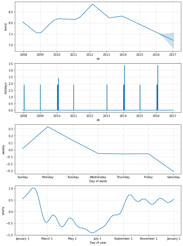
Individual holidays can be plotted using the plot_forecast_component function (imported from prophet.plot in Python) like plot_forecast_component(m, forecast, 'superbowl') to plot just the superbowl holiday component.
Built-in Country Holidays
You can use a built-in collection of country-specific holidays using the add_country_holidays method (Python) or function (R). The name of the country is specified, and then major holidays for that country will be included in addition to any holidays that are specified via the holidays argument described above:
1
2
3
4
# R
m <- prophet(holidays = holidays)
m <- add_country_holidays(m, country_name = 'US')
m <- fit.prophet(m, df)
1
2
3
4
# Python
m = Prophet(holidays=holidays)
m.add_country_holidays(country_name='US')
m.fit(df)
You can see which holidays were included by looking at the train_holiday_names (Python) or train.holiday.names (R) attribute of the model:
1
2
# R
m$train.holiday.names
1
2
3
4
5
6
7
8
 [1] "playoff"                     "superbowl"
 [3] "New Year's Day"              "Martin Luther King Jr. Day"
 [5] "Washington's Birthday"       "Memorial Day"
 [7] "Independence Day"            "Labor Day"
 [9] "Columbus Day"                "Veterans Day"
[11] "Veterans Day (Observed)"     "Thanksgiving"
[13] "Christmas Day"               "Independence Day (Observed)"
[15] "Christmas Day (Observed)"    "New Year's Day (Observed)"
1
2
# Python
m.train_holiday_names
1
2
3
4
5
6
7
8
9
10
11
12
13
14
15
16
17
0                         playoff
1                       superbowl
2                  New Year's Day
3      Martin Luther King Jr. Day
4           Washington's Birthday
5                    Memorial Day
6                Independence Day
7                       Labor Day
8                    Columbus Day
9                    Veterans Day
10                   Thanksgiving
11                  Christmas Day
12       Christmas Day (Observed)
13        Veterans Day (Observed)
14    Independence Day (Observed)
15      New Year's Day (Observed)
dtype: object
The holidays for each country are provided by the holidays package in Python. A list of available countries, and the country name to use, is available on their page: https://github.com/vacanza/python-holidays/.
In Python, most holidays are computed deterministically and so are available for any date range; a warning will be raised if dates fall outside the range supported by that country. In R, holiday dates are computed for 1995 through 2044 and stored in the package as data-raw/generated_holidays.csv. If a wider date range is needed, this script can be used to replace that file with a different date range: https://github.com/facebook/prophet/blob/main/python/scripts/generate_holidays_file.py.
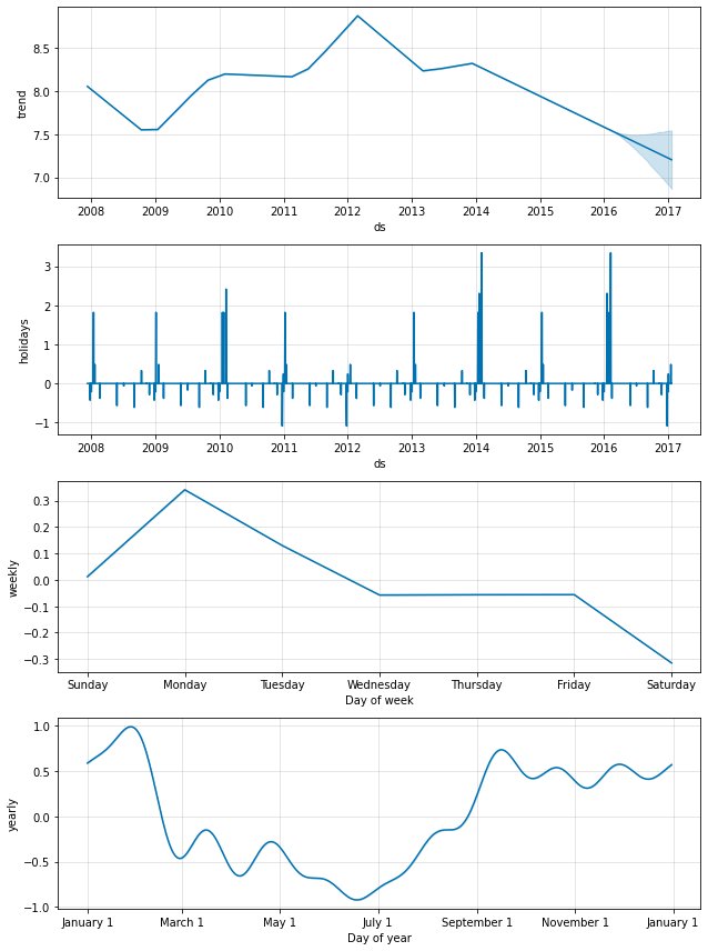
As above, the country-level holidays will then show up in the components plot:
1
2
3
# R
forecast <- predict(m, future)
prophet_plot_components(m, forecast)
1
2
3
# Python
forecast = m.predict(future)
fig = m.plot_components(forecast)
Holidays for subdivisions (Python)
We can use the utility function make_holidays_df to easily create custom holidays DataFrames, e.g. for certain states, using data from the holidays package. This can be passed directly to the Prophet() constructor.
1
2
3
4
5
6
7
# Python
from prophet.make_holidays import make_holidays_df

nsw_holidays = make_holidays_df(
    year_list=[2019 + i for i in range(10)], country='AU', province='NSW'
)
nsw_holidays.head(n=10)
| ds | holiday | |
|---|---|---|
| 0 | 2019-01-26 | Australia Day |
| 1 | 2019-01-28 | Australia Day (Observed) |
| 2 | 2019-04-25 | Anzac Day |
| 3 | 2019-12-25 | Christmas Day |
| 4 | 2019-12-26 | Boxing Day |
| 5 | 2019-04-20 | Easter Saturday |
| 6 | 2019-04-21 | Easter Sunday |
| 7 | 2019-10-07 | Labour Day |
| 8 | 2019-06-10 | Queen's Birthday |
| 9 | 2019-08-05 | Bank Holiday |
1
2
3
4
# Python
from prophet import Prophet

m_nsw = Prophet(holidays=nsw_holidays)
Fourier Order for Seasonalities
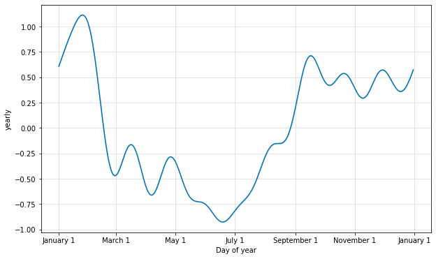
Seasonalities are estimated using a partial Fourier sum. See the paper for complete details, and this figure on Wikipedia for an illustration of how a partial Fourier sum can approximate an arbitrary periodic signal. The number of terms in the partial sum (the order) is a parameter that determines how quickly the seasonality can change. To illustrate this, consider the Peyton Manning data from the Quickstart. The default Fourier order for yearly seasonality is 10, which produces this fit:
1
2
3
# R
m <- prophet(df)
prophet:::plot_yearly(m)
1
2
3
4
# Python
from prophet.plot import plot_yearly
m = Prophet().fit(df)
a = plot_yearly(m)
The default values are often appropriate, but they can be increased when the seasonality needs to fit higher-frequency changes, and generally be less smooth. The Fourier order can be specified for each built-in seasonality when instantiating the model, here it is increased to 20:
1
2
3
# R
m <- prophet(df, yearly.seasonality = 20)
prophet:::plot_yearly(m)
1
2
3
4
# Python
from prophet.plot import plot_yearly
m = Prophet(yearly_seasonality=20).fit(df)
a = plot_yearly(m)
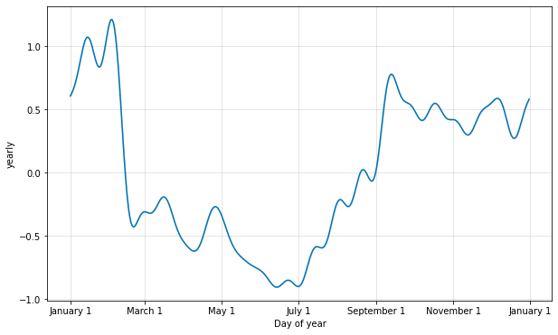
Increasing the number of Fourier terms allows the seasonality to fit faster changing cycles, but can also lead to overfitting: N Fourier terms corresponds to 2N variables used for modeling the cycle
Specifying Custom Seasonalities
Prophet will by default fit weekly and yearly seasonalities, if the time series is more than two cycles long. It will also fit daily seasonality for a sub-daily time series. You can add other seasonalities (monthly, quarterly, hourly) using the add_seasonality method (Python) or function (R).
The inputs to this function are a name, the period of the seasonality in days, and the Fourier order for the seasonality. For reference, by default Prophet uses a Fourier order of 3 for weekly seasonality and 10 for yearly seasonality. An optional input to add_seasonality is the prior scale for that seasonal component - this is discussed below.
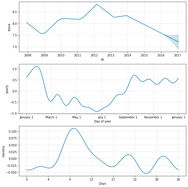
As an example, here we fit the Peyton Manning data from the Quickstart, but replace the weekly seasonality with monthly seasonality. The monthly seasonality then will appear in the components plot:
1
2
3
4
5
6
# R
m <- prophet(weekly.seasonality=FALSE)
m <- add_seasonality(m, name='monthly', period=30.5, fourier.order=5)
m <- fit.prophet(m, df)
forecast <- predict(m, future)
prophet_plot_components(m, forecast)
1
2
3
4
5
# Python
m = Prophet(weekly_seasonality=False)
m.add_seasonality(name='monthly', period=30.5, fourier_order=5)
forecast = m.fit(df).predict(future)
fig = m.plot_components(forecast)
Seasonalities that depend on other factors
In some instances the seasonality may depend on other factors, such as a weekly seasonal pattern that is different during the summer than it is during the rest of the year, or a daily seasonal pattern that is different on weekends vs. on weekdays. These types of seasonalities can be modeled using conditional seasonalities.
Consider the Peyton Manning example from the Quickstart. The default weekly seasonality assumes that the pattern of weekly seasonality is the same throughout the year, but we’d expect the pattern of weekly seasonality to be different during the on-season (when there are games every Sunday) and the off-season. We can use conditional seasonalities to construct separate on-season and off-season weekly seasonalities.
First we add a boolean column to the dataframe that indicates whether each date is during the on-season or the off-season:
1
2
3
4
5
6
7
8
# R
is_nfl_season <- function(ds) {
  dates <- as.Date(ds)
  month <- as.numeric(format(dates, '%m'))
  return(month > 8 | month < 2)
}
df$on_season <- is_nfl_season(df$ds)
df$off_season <- !is_nfl_season(df$ds)
1
2
3
4
5
6
7
# Python
def is_nfl_season(ds):
    date = pd.to_datetime(ds)
    return (date.month > 8 or date.month < 2)

df['on_season'] = df['ds'].apply(is_nfl_season)
df['off_season'] = ~df['ds'].apply(is_nfl_season)
Then we disable the built-in weekly seasonality, and replace it with two weekly seasonalities that have these columns specified as a condition. This means that the seasonality will only be applied to dates where the condition_name column is True. We must also add the column to the future dataframe for which we are making predictions.
1
2
3
4
5
6
7
8
9
10
# R
m <- prophet(weekly.seasonality=FALSE)
m <- add_seasonality(m, name='weekly_on_season', period=7, fourier.order=3, condition.name='on_season')
m <- add_seasonality(m, name='weekly_off_season', period=7, fourier.order=3, condition.name='off_season')
m <- fit.prophet(m, df)

future$on_season <- is_nfl_season(future$ds)
future$off_season <- !is_nfl_season(future$ds)
forecast <- predict(m, future)
prophet_plot_components(m, forecast)
1
2
3
4
5
6
7
8
9
# Python
m = Prophet(weekly_seasonality=False)
m.add_seasonality(name='weekly_on_season', period=7, fourier_order=3, condition_name='on_season')
m.add_seasonality(name='weekly_off_season', period=7, fourier_order=3, condition_name='off_season')

future['on_season'] = future['ds'].apply(is_nfl_season)
future['off_season'] = ~future['ds'].apply(is_nfl_season)
forecast = m.fit(df).predict(future)
fig = m.plot_components(forecast)
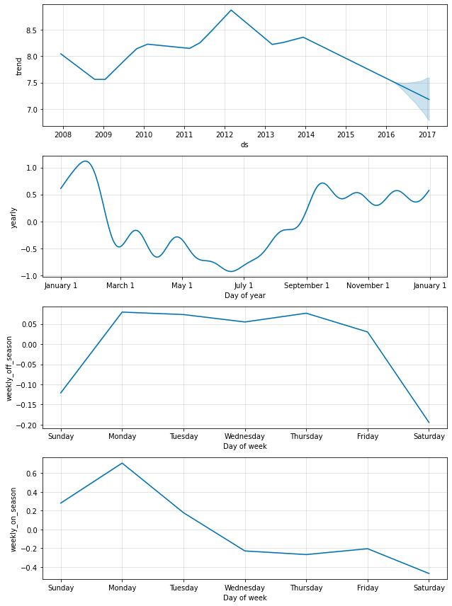
Both of the seasonalities now show up in the components plots above. We can see that during the on-season when games are played every Sunday, there are large increases on Sunday and Monday that are completely absent during the off-season.
Prior scale for holidays and seasonality
If you find that the holidays are overfitting, you can adjust their prior scale to smooth them using the parameter holidays_prior_scale. By default this parameter is 10, which provides very little regularization. Reducing this parameter dampens holiday effects:
1
2
3
4
5
6
7
# R
m <- prophet(df, holidays = holidays, holidays.prior.scale = 0.05)
forecast <- predict(m, future)
forecast %>%
  select(ds, playoff, superbowl) %>%
  filter(abs(playoff + superbowl) > 0) %>%
  tail(10)
1
2
3
4
5
# Python
m = Prophet(holidays=holidays, holidays_prior_scale=0.05).fit(df)
forecast = m.predict(future)
forecast[(forecast['playoff'] + forecast['superbowl']).abs() > 0][
    ['ds', 'playoff', 'superbowl']][-10:]
| ds | playoff | superbowl | |
|---|---|---|---|
| 2190 | 2014-02-02 | 1.206086 | 0.964914 |
| 2191 | 2014-02-03 | 1.852077 | 0.992634 |
| 2532 | 2015-01-11 | 1.206086 | 0.000000 |
| 2533 | 2015-01-12 | 1.852077 | 0.000000 |
| 2901 | 2016-01-17 | 1.206086 | 0.000000 |
| 2902 | 2016-01-18 | 1.852077 | 0.000000 |
| 2908 | 2016-01-24 | 1.206086 | 0.000000 |
| 2909 | 2016-01-25 | 1.852077 | 0.000000 |
| 2922 | 2016-02-07 | 1.206086 | 0.964914 |
| 2923 | 2016-02-08 | 1.852077 | 0.992634 |
The magnitude of the holiday effect has been reduced compared to before, especially for superbowls, which had the fewest observations. There is a parameter seasonality_prior_scale which similarly adjusts the extent to which the seasonality model will fit the data.
Prior scales can be set separately for individual holidays by including a column prior_scale in the holidays dataframe. Prior scales for individual seasonalities can be passed as an argument to add_seasonality. For instance, the prior scale for just weekly seasonality can be set using:
1
2
3
4
# R
m <- prophet()
m <- add_seasonality(
  m, name='weekly', period=7, fourier.order=3, prior.scale=0.1)
1
2
3
4
# Python
m = Prophet()
m.add_seasonality(
    name='weekly', period=7, fourier_order=3, prior_scale=0.1)
Additional regressors
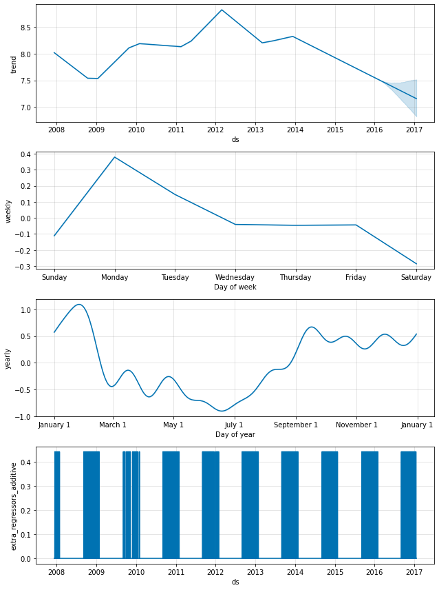
Additional regressors can be added to the linear part of the model using the add_regressor method or function. A column with the regressor value will need to be present in both the fitting and prediction dataframes. For example, we can add an additional effect on Sundays during the NFL season. On the components plot, this effect will show up in the ‘extra_regressors’ plot:
1
2
3
4
5
6
7
8
9
10
11
12
13
14
15
16
# R
nfl_sunday <- function(ds) {
  dates <- as.Date(ds)
  month <- as.numeric(format(dates, '%m'))
  as.numeric((weekdays(dates) == "Sunday") & (month > 8 | month < 2))
}
df$nfl_sunday <- nfl_sunday(df$ds)

m <- prophet()
m <- add_regressor(m, 'nfl_sunday')
m <- fit.prophet(m, df)

future$nfl_sunday <- nfl_sunday(future$ds)

forecast <- predict(m, future)
prophet_plot_components(m, forecast)
1
2
3
4
5
6
7
8
9
10
11
12
13
14
15
16
17
# Python
def nfl_sunday(ds):
    date = pd.to_datetime(ds)
    if date.weekday() == 6 and (date.month > 8 or date.month < 2):
        return 1
    else:
        return 0
df['nfl_sunday'] = df['ds'].apply(nfl_sunday)

m = Prophet()
m.add_regressor('nfl_sunday')
m.fit(df)

future['nfl_sunday'] = future['ds'].apply(nfl_sunday)

forecast = m.predict(future)
fig = m.plot_components(forecast)
NFL Sundays could also have been handled using the “holidays” interface described above, by creating a list of past and future NFL Sundays. The add_regressor function provides a more general interface for defining extra linear regressors, and in particular does not require that the regressor be a binary indicator. Another time series could be used as a regressor, although its future values would have to be known.
This notebook shows an example of using weather factors as extra regressors in a forecast of bicycle usage, and provides an excellent illustration of how other time series can be included as extra regressors.
The add_regressor function has optional arguments for specifying the prior scale (holiday prior scale is used by default) and whether or not the regressor is standardized - see the docstring with help(Prophet.add_regressor) in Python and ?add_regressor in R. Note that regressors must be added prior to model fitting. Prophet will also raise an error if the regressor is constant throughout the history, since there is nothing to fit from it.
The extra regressor must be known for both the history and for future dates. It thus must either be something that has known future values (such as nfl_sunday), or something that has separately been forecasted elsewhere. The weather regressors used in the notebook linked above is a good example of an extra regressor that has forecasts that can be used for future values.
One can also use as a regressor another time series that has been forecasted with a time series model, such as Prophet. For instance, if r(t) is included as a regressor for y(t), Prophet can be used to forecast r(t) and then that forecast can be plugged in as the future values when forecasting y(t). A note of caution around this approach: This will probably not be useful unless r(t) is somehow easier to forecast than y(t). This is because error in the forecast of r(t) will produce error in the forecast of y(t). One setting where this can be useful is in hierarchical time series, where there is top-level forecast that has higher signal-to-noise and is thus easier to forecast. Its forecast can be included in the forecast for each lower-level series.
Extra regressors are put in the linear component of the model, so the underlying model is that the time series depends on the extra regressor as either an additive or multiplicative factor (see the next section for multiplicativity).
Coefficients of additional regressors
To extract the beta coefficients of the extra regressors, use the utility function regressor_coefficients (from prophet.utilities import regressor_coefficients in Python, prophet::regressor_coefficients in R) on the fitted model. The estimated beta coefficient for each regressor roughly represents the increase in prediction value for a unit increase in the regressor value (note that the coefficients returned are always on the scale of the original data). If mcmc_samples is specified, a credible interval for each coefficient is also returned, which can help identify whether the regressor is meaningful to the model (a credible interval that includes the 0 value suggests the regressor is not meaningful).