
Quick Start
Python API
Prophet follows the sklearn model API. We create an instance of the Prophet class and then call its fit and predict methods.
The input to Prophet is always a dataframe with two columns: ds and y. The ds (datestamp) column should be of a format expected by Pandas, ideally YYYY-MM-DD for a date or YYYY-MM-DD HH:MM:SS for a timestamp. The y column must be numeric, and represents the measurement we wish to forecast.
As an example, let’s look at a time series of the log daily page views for the Wikipedia page for Peyton Manning. We scraped this data using the Wikipediatrend package in R. Peyton Manning provides a nice example because it illustrates some of Prophet’s features, like multiple seasonality, changing growth rates, and the ability to model special days (such as Manning’s playoff and superbowl appearances). The CSV is available here.
First we’ll import the data:
1
2
3
4
# Python
import pandas as pd
from prophet import Prophet
1
2
3
4
# Python
df = pd.read_csv('https://raw.githubusercontent.com/facebook/prophet/main/examples/example_wp_log_peyton_manning.csv')
df.head()
| ds | y | |
|---|---|---|
| 0 | 2007-12-10 | 9.590761 |
| 1 | 2007-12-11 | 8.519590 |
| 2 | 2007-12-12 | 8.183677 |
| 3 | 2007-12-13 | 8.072467 |
| 4 | 2007-12-14 | 7.893572 |
We fit the model by instantiating a new Prophet object. Any settings to the forecasting procedure are passed into the constructor. Then you call its fit method and pass in the historical dataframe. Fitting should take 1-5 seconds.
1
2
3
4
# Python
m = Prophet()
m.fit(df)
Predictions are then made on a dataframe with a column ds containing the dates for which a prediction is to be made. You can get a suitable dataframe that extends into the future a specified number of days using the helper method Prophet.make_future_dataframe. By default it will also include the dates from the history, so we will see the model fit as well.
1
2
3
4
# Python
future = m.make_future_dataframe(periods=365)
future.tail()
| ds | |
|---|---|
| 3265 | 2017-01-15 |
| 3266 | 2017-01-16 |
| 3267 | 2017-01-17 |
| 3268 | 2017-01-18 |
| 3269 | 2017-01-19 |
The predict method will assign each row in future a predicted value which it names yhat. If you pass in historical dates, it will provide an in-sample fit. The forecast object here is a new dataframe that includes a column yhat with the forecast, as well as columns for components and uncertainty intervals.
1
2
3
4
# Python
forecast = m.predict(future)
forecast[['ds', 'yhat', 'yhat_lower', 'yhat_upper']].tail()
| ds | yhat | yhat_lower | yhat_upper | |
|---|---|---|---|---|
| 3265 | 2017-01-15 | 8.212625 | 7.456310 | 8.959726 |
| 3266 | 2017-01-16 | 8.537635 | 7.842986 | 9.290934 |
| 3267 | 2017-01-17 | 8.325071 | 7.600879 | 9.072006 |
| 3268 | 2017-01-18 | 8.157723 | 7.512052 | 8.924022 |
| 3269 | 2017-01-19 | 8.169677 | 7.412473 | 8.946977 |
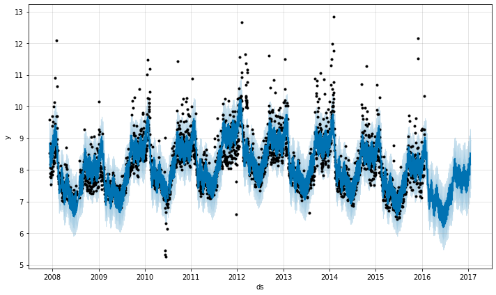
You can plot the forecast by calling the Prophet.plot method and passing in your forecast dataframe.
1
2
3
# Python
fig1 = m.plot(forecast)
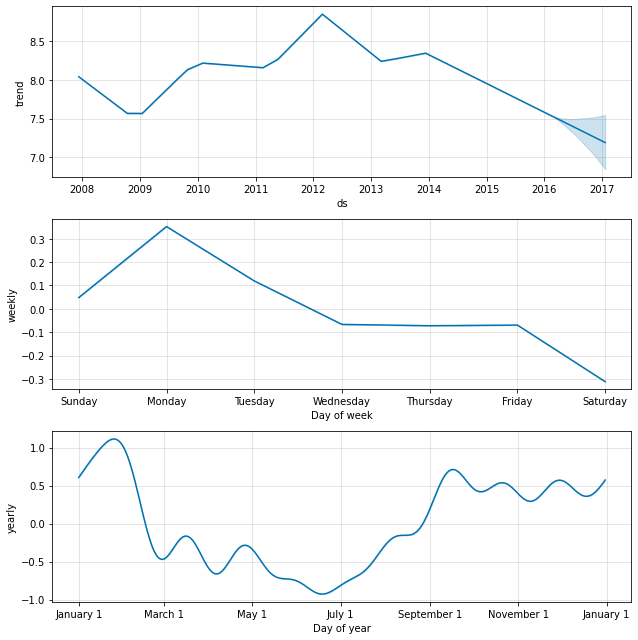
If you want to see the forecast components, you can use the Prophet.plot_components method. By default you’ll see the trend, yearly seasonality, and weekly seasonality of the time series. If you include holidays, you’ll see those here, too.
1
2
3
# Python
fig2 = m.plot_components(forecast)
An interactive figure of the forecast and components can be created with plotly. You will need to install plotly 4.0 or above separately, as it will not by default be installed with prophet. You will also need to install the notebook and ipywidgets packages.
1
2
3
4
5
# Python
from prophet.plot import plot_plotly, plot_components_plotly

plot_plotly(m, forecast)
1
2
3
# Python
plot_components_plotly(m, forecast)
More details about the options available for each method are available in the docstrings, for example, via help(Prophet) or help(Prophet.fit).
R API
In R, we use the normal model fitting API. We provide a prophet function that performs fitting and returns a model object. You can then call predict and plot on this model object.
1
2
3
# R
library(prophet)
1
2
3
R[write to console]: Loading required package: Rcpp

R[write to console]: Loading required package: rlang
First we read in the data and create the outcome variable. As in the Python API, this is a dataframe with columns ds and y, containing the date and numeric value respectively. The ds column should be YYYY-MM-DD for a date, or YYYY-MM-DD HH:MM:SS for a timestamp. As above, we use here the log number of views to Peyton Manning’s Wikipedia page, available here.
1
2
3
# R
df <- read.csv('https://raw.githubusercontent.com/facebook/prophet/main/examples/example_wp_log_peyton_manning.csv')
We call the prophet function to fit the model. The first argument is the historical dataframe. Additional arguments control how Prophet fits the data and are described in later pages of this documentation.
1
2
3
# R
m <- prophet(df)
Predictions are made on a dataframe with a column ds containing the dates for which predictions are to be made. The make_future_dataframe function takes the model object and a number of periods to forecast and produces a suitable dataframe. By default it will also include the historical dates so we can evaluate in-sample fit.
1
2
3
4
# R
future <- make_future_dataframe(m, periods = 365)
tail(future)
1
2
3
4
5
6
7
             ds
3265 2017-01-14
3266 2017-01-15
3267 2017-01-16
3268 2017-01-17
3269 2017-01-18
3270 2017-01-19
As with most modeling procedures in R, we use the generic predict function to get our forecast. The forecast object is a dataframe with a column yhat containing the forecast. It has additional columns for uncertainty intervals and seasonal components.
1
2
3
4
# R
forecast <- predict(m, future)
tail(forecast[c('ds', 'yhat', 'yhat_lower', 'yhat_upper')])
1
2
3
4
5
6
7
             ds     yhat yhat_lower yhat_upper
3265 2017-01-14 7.818359   7.071228   8.550957
3266 2017-01-15 8.200125   7.475725   8.869495
3267 2017-01-16 8.525104   7.747071   9.226915
3268 2017-01-17 8.312482   7.551904   9.046774
3269 2017-01-18 8.145098   7.390770   8.863692
3270 2017-01-19 8.156964   7.381716   8.866507
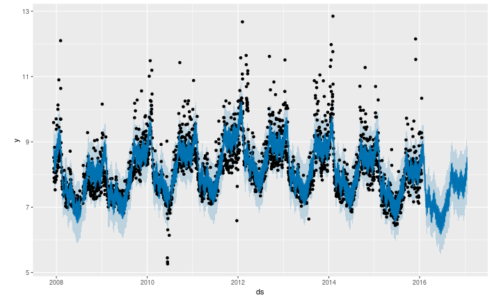
You can use the generic plot function to plot the forecast, by passing in the model and the forecast dataframe.
1
2
3
# R
plot(m, forecast)
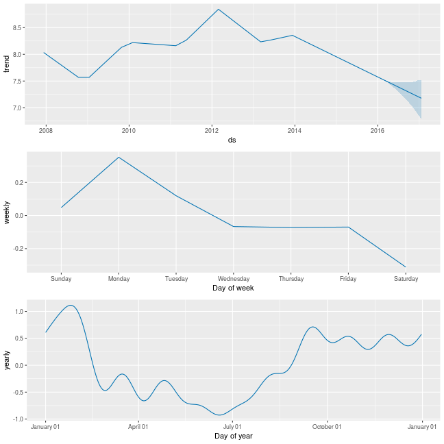
You can use the prophet_plot_components function to see the forecast broken down into trend, weekly seasonality, and yearly seasonality.
1
2
3
# R
prophet_plot_components(m, forecast)
An interactive plot of the forecast using Dygraphs can be made with the command dyplot.prophet(m, forecast).
More details about the options available for each method are available in the docstrings, for example, via ?prophet or ?fit.prophet. This documentation is also available in the reference manual on CRAN.